

![]()
Paste Tools: Several tools for pasting information from the Clipboard as pictures (video overview)
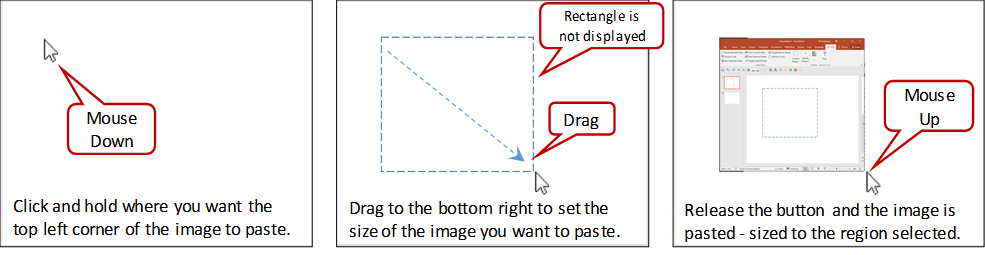
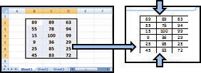
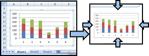
![]() Paste to Size: Pastes the contents from the clipboard to fit the selected region. The dimensions are constrained by the ratios between the height and width of the region and the height and width of the clipboard content. The clipboard contents are pasted as an enhanced meta file.
Paste to Size: Pastes the contents from the clipboard to fit the selected region. The dimensions are constrained by the ratios between the height and width of the region and the height and width of the clipboard content. The clipboard contents are pasted as an enhanced meta file.
![]() Paste To Height: Pastes the contents of the clipboard to the top left cell of the selected range and resizes it to the height of the range. Command also available as a “right click” menu item.
Paste To Height: Pastes the contents of the clipboard to the top left cell of the selected range and resizes it to the height of the range. Command also available as a “right click” menu item.

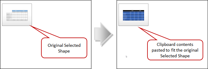
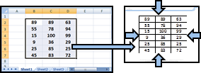
![]() Paste Replace: Pastes the contents from the clipboard to fit the selected shape’s height or width based on the ratio and deletes the original shape – effectively replacing the original shape. The dimensions are constrained by the ratios between the height and width of the original shape and the height and width of the clipboard content. The clipboard contents are pasted as an enhanced meta file.
Paste Replace: Pastes the contents from the clipboard to fit the selected shape’s height or width based on the ratio and deletes the original shape – effectively replacing the original shape. The dimensions are constrained by the ratios between the height and width of the original shape and the height and width of the clipboard content. The clipboard contents are pasted as an enhanced meta file.
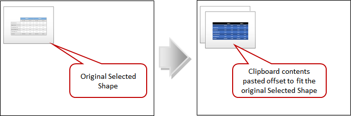
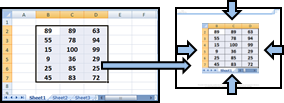
![]() Paste Offset: Pastes the contents from the clipboard to fit the selected shape’s height or width based on the ratio – with an offset. The dimensions are constrained by the ratios between the height and width of the original shape and the height and width of the clipboard content. The clipboard contents are pasted as an enhanced meta file.
Paste Offset: Pastes the contents from the clipboard to fit the selected shape’s height or width based on the ratio – with an offset. The dimensions are constrained by the ratios between the height and width of the original shape and the height and width of the clipboard content. The clipboard contents are pasted as an enhanced meta file.
Print Tools: Three simple printing tools.
![]() Print Range: Based on the selected range, prints the selection scaled to fit a single page.
Print Range: Based on the selected range, prints the selection scaled to fit a single page.

![]() Print Sheet: Based on the Page Setup, prints the current Sheet.
Print Sheet: Based on the Page Setup, prints the current Sheet.

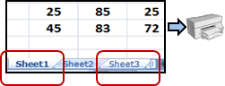
![]() Print Sheets: Based on the Page Setup, prints the currently selected Sheets.
Print Sheets: Based on the Page Setup, prints the currently selected Sheets.
Worksheet Tools: A series of tools for formatting and adding custom charts / forms. (video overview)
![]() Navigator: The Navigator provides a number of functions to work with and move between open Workbooks and their associated Worksheets. Note: The Navigator does not function with Workbooks with multiple document windows in the same Workbook.
Navigator: The Navigator provides a number of functions to work with and move between open Workbooks and their associated Worksheets. Note: The Navigator does not function with Workbooks with multiple document windows in the same Workbook.
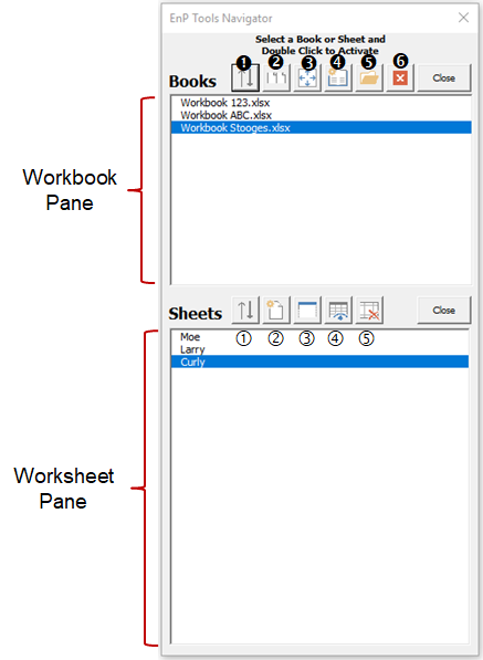
When opened, the Navigator displays all currently opened Workbooks in the Workbook Pane. The active Workbook is selected and the visible Worksheets are displayed in the Worksheet Pane with the active Worksheet selected. To display a different Workbook or Worksheet, select the appropriate item and then double click. The Navigator will display the selected Workbook or Worksheet.
Workbook Functions:
❶ Sort Workbooks: Sorts the list of Workbooks in the Workbook Pane – Ascending or Descending.
❷ View 2 Workbooks: Displays the active Workbook and one other highlighted Workbook – Side by Side. The other workbooks are minimized.
❸ Stretch Across Monitors: Essentially maximizes the active Workbook across multiple monitors.
❹ New Workbook: Opens and New Workbook and activates it.
❺ Open Workbook: Opens a file dialog to choose another Workbook to open. It makes it the active Workbook.
❻ Close Workbook: Closes the highlighted Workbook. If the highlighted Workbook is the active workbook, no action is taken.
Close: Closes the Navigator form.
Worksheet Functions:
① Sort Worksheets: Sorts the list of Workbooks in the Workbook Pane – Ascending or Descending and the actual Worksheets in the Workbook.
② New Worksheet: Adds a New Worksheet after the currently selected Worksheet and activates it.
③ Hide Worksheet: Hides the currently highlighted Worksheet.
④ Unhide All Worksheets: Unhides all hidden Worksheets in the active Workbook.
⑤ Delete Worksheet: Deletes the highlighted Worksheet.Close: Closes the Navigator form.
![]() Data Prep: 42 Tools to assist in preparing data for processing including 3 built-in Excel functions – Text to Columns, Flash Fill & Spell Check.
Data Prep: 42 Tools to assist in preparing data for processing including 3 built-in Excel functions – Text to Columns, Flash Fill & Spell Check.
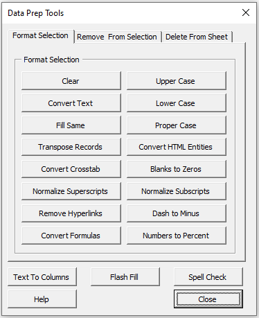
Clear: Clears all formatting from the selected Range
Convert Text: Converts formatting to General e.g. a date entered as Text will be converted Date. Clicking again will convert it to the date serial.
Fill Same: Fills blank cells with the value above in the selected range. Merged cell are split up.
Transpose Records: Transposes columnar records based on user input to the left inserting the appropriate number of columns.![]()
Convert Crosstab: Converts Crosstab Tables (2-Dimensional Tables) To Lists. The Crosstab can be a range or table; however, the first row must contain headers. The range must be separated from other data. The User is prompted to enter the number of columns on the left that will be used to create the list columns. The remaining rows in the Crosstab will be “unpivoted”. The resulting list is placed in a table on a new worksheet.
Normalize Superscripts: Converts Superscript characters to Normal in the Selection.
Remove Hyperlinks: Removes Hyperlinks in the Selection.
Convert Formulas: Converts formulas to values in the current selection.
Upper Case: Converts the text to upper case in the selected cells.
Lower Case: Converts the text to lower case in the selected cells.
Proper Case: Converts the text to proper case in the selected cells.
Convert HTML Entities: Convert HTML Entities such as: &lt;tag&gt; to <tag>
Blanks to Zeros: In the selected range, adds zeros to blank cells.
Normalize Subscripts: Converts Subscript characters to Normal in the Selection.
Dash to Minus: Converts Dashes and Hyphens to Minus signs.
U+2010 Hyphen
U+2011 Non-Beaking Hyphen
U+2012 Figure Dash
U+2013 En Dash
U+2014 Em Dash
Numbers to Percent: Converts Numbers to Percent by dividing by 100 and formating as Percent. e.g. 10 becomes 10.0%. Note: Formulas are converted to values.

Non-visible Characters: Removes non-visible characters such as Tab and replaces nonbreaking space characters with space from the selection.
Extra Spaces: Removes extra spaces from the selection – basically Excel’s TRIM() function.
Double Quotes: Removes double quotes from the selection.
Single Quotes: Removes single quotes from the selection.
Superscript Chars: Removes Superscript Characters from the selection.
Before Nth Char: Removes the string before the nth character inputted into the textbox. e.g. 9 returns Test.xlsx from C:\Temp\Test.xlsx
After Nth Char: Removes the string after the nth character inputted into the textbox. e.g. 7 returns C:\Temp from C:\Temp\Test.xlsx
Specific Character: Removes the single character inputted into the textbox from the selected text.
Punctuation: Removes punctuation from the selection.
Numbers: Removes numbers from the selection.
Letters: Removes letters from the selection.
Subscript Chars: Removes Subscript Characters from the selection.
Shapes and Images: Removes Superscript Characters from the selection.
Before Character: Removes the string before the character inputted into the textbox
e.g. entering \ results in Temp\Test.xlsx from C:\Temp\Test.xlsx
After Character: Removes the string after the character inputted into the textbox as well as the character.
e.g. entering \ results in C:\ from C:\Temp\Test.xlsx.

Hidden Rows: Deletes all hidden rows on the sheet.
Empty Rows: Deletes all empty rows on the sheet.
Rows with only 1 Entry: Deletes all rows with only 1 entry. Can useful when importing text files with page header/footer rows.
Every Nth Row: Deletes every nth row specified by the User in the current selection.
Hidden Columns: Deletes all hidden columns on the sheet.
Empty Columns: Deletes all empty columns on the sheet.
Columns with only 1 Entry: Deletes all Columns with only 1 entry. Useful if column has a header but no data.
Every Nth Column: Deletes every nth column specified by the User in the current selection.
Duplicate Rows: Delete or Find Duplicate Rows based on Values from Column(s). Data to be checked must start in Cell A1.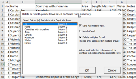
1) Select the columns that determine duplicate rows.
2) Confirm if the data has a Header row – default is yes. If unchecked, a Header row is inserted with values Data1, Data2, etc…
3) Match Case if the data to be compared is case sensitive.
4) Confirm that duplicates are to be deleted – this keeps only the first row in multiple groups. The default is yes. If unchecked, duplicate rows are grouped together and highlighted.
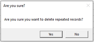
5) A number of messages appear as the process is completed:

6) Results appear as such
Charting Tools
![]() Add Waterfall Chart: From the selection of a horizontal range (titles and values), adds a sheet with a Waterfall or Step Down Graph. Selected range must be 2 rows and at least 2 columns. The final column’s title cannot be a number. The final column value will be recalculated. Buttons on the sheet allow the user to
Add Waterfall Chart: From the selection of a horizontal range (titles and values), adds a sheet with a Waterfall or Step Down Graph. Selected range must be 2 rows and at least 2 columns. The final column’s title cannot be a number. The final column value will be recalculated. Buttons on the sheet allow the user to
- Cycle Data Label Formats – 0 to 4 decimal places, $ and $0.00
- Set Labels Above – resets the labels if the values are manually changed in the sheets. It also re-sync’s the hidden secondary axis for the segment values.
- Reverse Colours – toggles colours between green and red e.g. if negative change is favourable.


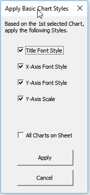
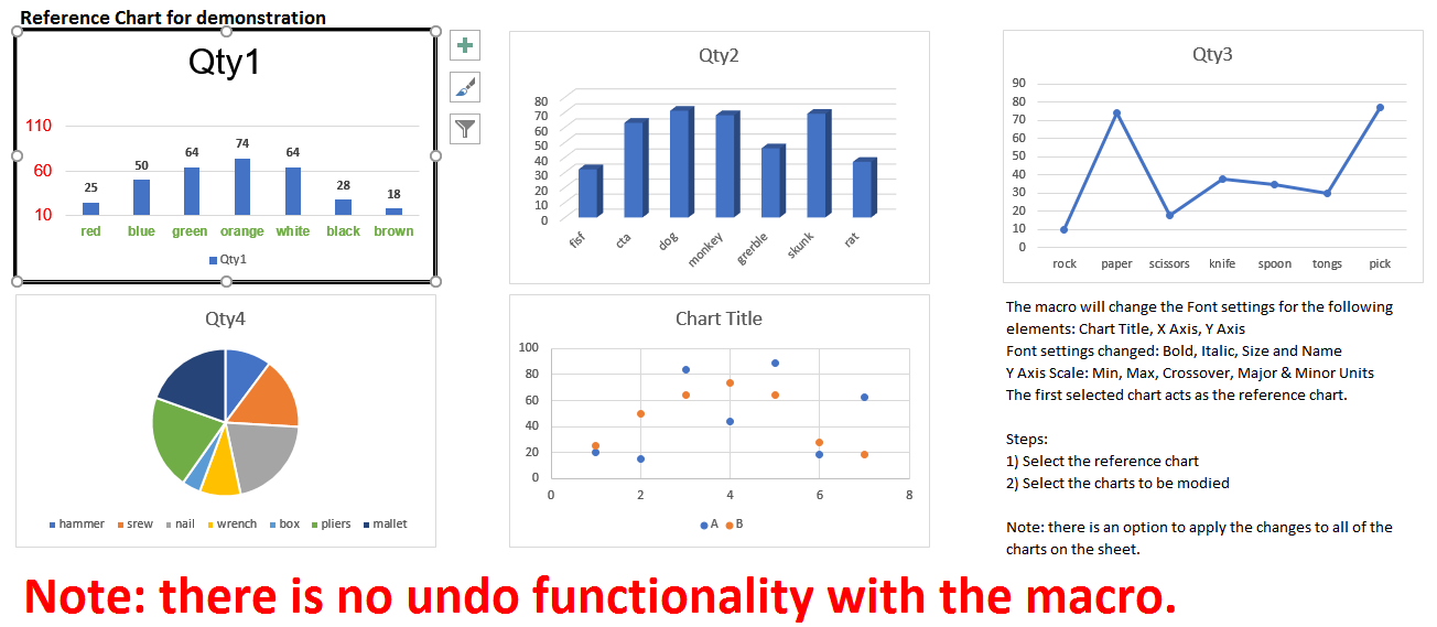
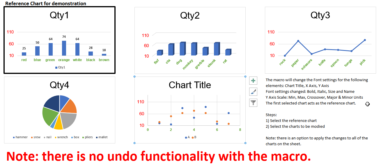
![]() Basic Chart Formatter: Based on the first selected chart, other charts’ settings can be changed. The Font settings for the following elements can be changed: Chart Title, X Axis, Y Axis. Font settings changed: Bold, Italic, Size and Name. Also, the Y Axis Scale: Min, Max, Crossover, Major and Minor Units can be copied and applied. The user can choose which elements to copy and choose between selected charts or all charts on the worksheet.
Basic Chart Formatter: Based on the first selected chart, other charts’ settings can be changed. The Font settings for the following elements can be changed: Chart Title, X Axis, Y Axis. Font settings changed: Bold, Italic, Size and Name. Also, the Y Axis Scale: Min, Max, Crossover, Major and Minor Units can be copied and applied. The user can choose which elements to copy and choose between selected charts or all charts on the worksheet.

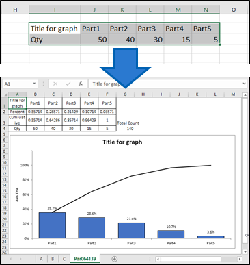
![]() Create Basic Pareto Chart: Based on user selected range, creates a simple Pareto Chart using frequency and cumulative frequency. Cell A1 is linked with the chart’s title.
Create Basic Pareto Chart: Based on user selected range, creates a simple Pareto Chart using frequency and cumulative frequency. Cell A1 is linked with the chart’s title.
![]() Create Dot Chart: Based on user selected range, creates a vertical Dot Chart. The user must select 2 columns and at least 2 rows. The first row is considered a header row.
Create Dot Chart: Based on user selected range, creates a vertical Dot Chart. The user must select 2 columns and at least 2 rows. The first row is considered a header row.

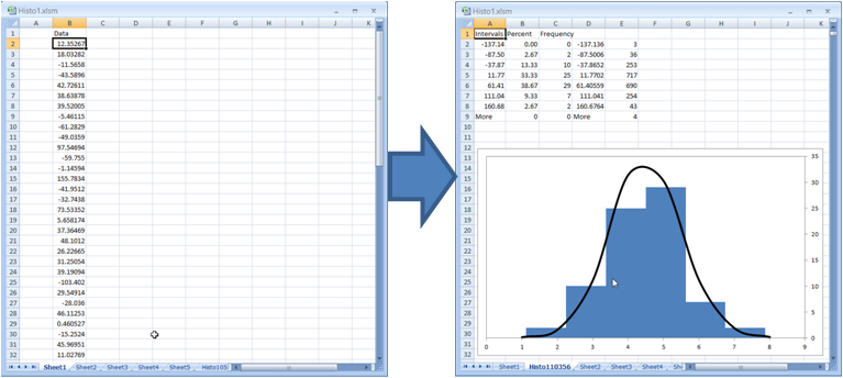
![]() Create Basic Histogram: Based on the selected cell down, creates a basic Histogram. The chart’s intervals are fixed to 8 and the interval size is based on the data’s standard deviation. The accompanying Bell shaped curved is based on 2000 “random” numbers with the same standard deviation and mean value as the data from the histogram.
Create Basic Histogram: Based on the selected cell down, creates a basic Histogram. The chart’s intervals are fixed to 8 and the interval size is based on the data’s standard deviation. The accompanying Bell shaped curved is based on 2000 “random” numbers with the same standard deviation and mean value as the data from the histogram.
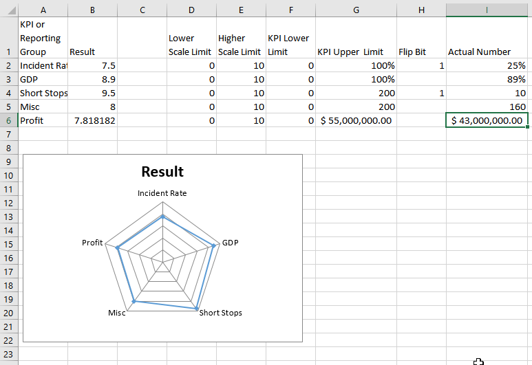
![]() Create Normalized Radar Chart: Based on the range selected, creates a Radar chart with data normalized to a scale of 10.
Create Normalized Radar Chart: Based on the range selected, creates a Radar chart with data normalized to a scale of 10.
The following (linear) equations can be applied to any number x in the A-B range:
y = C + (x-A)*(D-C)/(B-A) or y =D-(C + (x-A)*(D-C)/(B-A) )
where
A = the upper range limit
B = the upper range limit
C = the lower scale limit
D = the upper scale limit
The “Flip Bit” is used to adjust the Actual Normalized Number when the smaller the Actual Number is, more favourable it is – as in the case of Safety Incidents. It adjusts the smallest number to be the number closet to 10 i.e. the most favourable. Use 1 as the Flip Bit value when required; otherwise, leave it blank.
The data must be arranged as below (5 columns and at least 3 rows including a title row). The titles can be changed to whatever. Mandatory fields – KPI Limits & Actual Numbers. These can be rates, dollar amounts, integers, etc…

A Sheet is added and a chart with the normalized results is created as shown below. Data can be modified on this sheet.
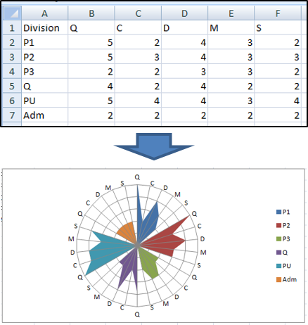
P Create Petal Chart: Based on user selected range, creates a modified radar chart to compare groups with specific categories. The Petal Chart can provide a clear visual comparison between different groups.
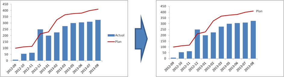
![]() Create Plan vs Actual Chart: Based on user selected 3 row range, creates a simple Plan vs Actual Chart. The columns’ colours are set are automatically: Green for favourable to target and Red for unfavourable. Cell A1 is linked with the chart’s title.
Create Plan vs Actual Chart: Based on user selected 3 row range, creates a simple Plan vs Actual Chart. The columns’ colours are set are automatically: Green for favourable to target and Red for unfavourable. Cell A1 is linked with the chart’s title.
Buttons on the sheet allow the user to
- Cycle Data Label Formats – 0 to 4 decimal places, $ and $0.00
- Reverse Colours – toggles colours between green and red e.g. if negative change is favourable.

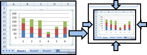
![]() Create Simple Chart: Select the chart to copy, size and “simplify”. A dialog box prompts the user to select a range. The chart is copied and sized to fit the range. Most Chart elements are removed to leave just the data series. The simplified chart remains linked to the data source.
Create Simple Chart: Select the chart to copy, size and “simplify”. A dialog box prompts the user to select a range. The chart is copied and sized to fit the range. Most Chart elements are removed to leave just the data series. The simplified chart remains linked to the data source.

![]() Create T Chart: Based on user selected range, creates a modified stacked bar chart to compare positive and negative changes. Useful for creating comparisons between categories that improved or worsened. Colours can be switched based on user requirements. The third column is used to locate the x axis labels. Works best with integers.
Create T Chart: Based on user selected range, creates a modified stacked bar chart to compare positive and negative changes. Useful for creating comparisons between categories that improved or worsened. Colours can be switched based on user requirements. The third column is used to locate the x axis labels. Works best with integers.

![]() Label Line Last Data Point: Select the chart to modify. A label will be placed to the right of the last data point of any line series and the Legend (if any) will be removed.
Label Line Last Data Point: Select the chart to modify. A label will be placed to the right of the last data point of any line series and the Legend (if any) will be removed.
![]() Move and Size Chart: Select the chart to move and size. A dialog box prompts the user to select a range. The chart is moved and sized to fit the range.
Move and Size Chart: Select the chart to move and size. A dialog box prompts the user to select a range. The chart is moved and sized to fit the range.

 Formatting Tools
![]() Change Case: Changes the Case of the selected Range – except cells with formulas – based on the user choice.
Change Case: Changes the Case of the selected Range – except cells with formulas – based on the user choice.

![]() Column to Multi-Column: Adds a new Sheet with information distributed into the number of required columns based on the selected cells in a column and the inputted number of columns.
Column to Multi-Column: Adds a new Sheet with information distributed into the number of required columns based on the selected cells in a column and the inputted number of columns.

![]() Copy Rows Below: Copies and inserts the selected rows below the current selection. Rows, cells or ranges can be selected. This is particularly useful to add new rows to an SAP.
Copy Rows Below: Copies and inserts the selected rows below the current selection. Rows, cells or ranges can be selected. This is particularly useful to add new rows to an SAP.
![]() Concatenate Range: Inserts the function – EnPConcat which concatenates a range of cells using an optional delimiter.
Concatenate Range: Inserts the function – EnPConcat which concatenates a range of cells using an optional delimiter.
Delimiter (Optional): user defined separator between elements.
AsShown (Optional): False displays actual values (default) while True displays the text as formatted.
OmitBlanks (Optional: True omits blanks cells while False includes them (default).

![]() Cycle Fill Colours: Cycles the fill colours of the selected shapes through Light Blue, Dark Blue, Light Grey, Orange and White.
Cycle Fill Colours: Cycles the fill colours of the selected shapes through Light Blue, Dark Blue, Light Grey, Orange and White.

![]() Delete Hidden Rows: Deletes all the hidden rows on the active sheet. Particularly useful when using auto filter.
Delete Hidden Rows: Deletes all the hidden rows on the active sheet. Particularly useful when using auto filter.

![]() Fill Same: Fills blank cells with the value above in the selected range. Works best with values not formulas. Use the Formula to Value tool in Misc Tools to convert formulas to values.
Fill Same: Fills blank cells with the value above in the selected range. Works best with values not formulas. Use the Formula to Value tool in Misc Tools to convert formulas to values.

![]() Format Range: Applies borders and alternating rows fills to the current Selection.
Format Range: Applies borders and alternating rows fills to the current Selection.

![]() Hide Shapes: Tools to hide and unhide shapes (circles, textboxes, tables, etc…) throughout the Workbook. Shapes must be Tags first.
Hide Shapes: Tools to hide and unhide shapes (circles, textboxes, tables, etc…) throughout the Workbook. Shapes must be Tags first.
![]() Add Hidden Tags: Adds the suffix “_Hide” to the Name of the selected shapes to enable the Hide Unhide functionality.
Add Hidden Tags: Adds the suffix “_Hide” to the Name of the selected shapes to enable the Hide Unhide functionality.
![]() Hide Unhide Shapes: Hides or Unhides Shapes with Names that have the suffix “_Hide” throughout the Workbook.
Hide Unhide Shapes: Hides or Unhides Shapes with Names that have the suffix “_Hide” throughout the Workbook.
![]() Remove Hidden Tags: Removes the suffix “_Hide” where applied and Unhides those Shapes if Hidden throughout the Workbook.
Remove Hidden Tags: Removes the suffix “_Hide” where applied and Unhides those Shapes if Hidden throughout the Workbook.
![]() Unhide All Shapes: Unhides all Shapes in the Workbook keeping any Names with the suffix “_Hide” assigned.
Unhide All Shapes: Unhides all Shapes in the Workbook keeping any Names with the suffix “_Hide” assigned.
![]() Highlight Alternate Rows: Highlights alternate rows within the Selected Range.
Highlight Alternate Rows: Highlights alternate rows within the Selected Range.
![]() Highlight Duplicate Cells: Highlights cells within a selected range if there are duplicates.
Highlight Duplicate Cells: Highlights cells within a selected range if there are duplicates.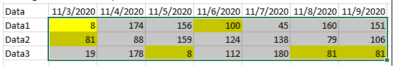
![]() Highlight Duplicates by Value: Highlights cells within a selected range based on a cell in the range. An Input Box is used to select the source cell for the comparison. If only 1 cell is found with the value, the cell is highlighted in Blue. Otherwise, found values are highlighted in Green.
Highlight Duplicates by Value: Highlights cells within a selected range based on a cell in the range. An Input Box is used to select the source cell for the comparison. If only 1 cell is found with the value, the cell is highlighted in Blue. Otherwise, found values are highlighted in Green.
![]() Highlight Formulas: Highlights cells with formulas in a selected range.
Highlight Formulas: Highlights cells with formulas in a selected range.
![]() Highlight Max Min: Highlights the max and min values in a selected range.
Highlight Max Min: Highlights the max and min values in a selected range.
![]() Highlight Named Ranges: Highlights all named ranges in the workbook.
Highlight Named Ranges: Highlights all named ranges in the workbook.
![]() Highlight Unique: Highlights cells with unique values in a selected range. The highlighting is accomplished with conditional formatting.
Highlight Unique: Highlights cells with unique values in a selected range. The highlighting is accomplished with conditional formatting.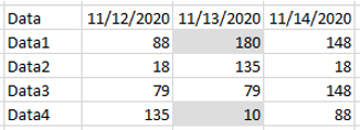
![]() Highlight Remove: Sets the cell fill colour to none in the selected range.
Highlight Remove: Sets the cell fill colour to none in the selected range.
![]() Insert Empty Columns: Within the selected range, inserts an empty column after every nth column as specified by the user.
Insert Empty Columns: Within the selected range, inserts an empty column after every nth column as specified by the user.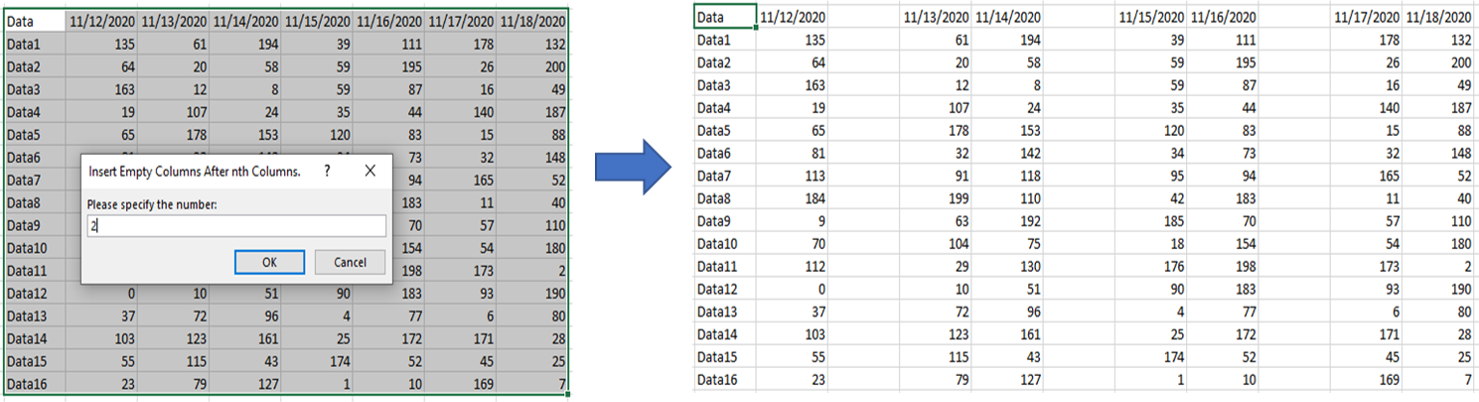
![]() Insert Empty Rows: Within the selected range, inserts an empty row after every nth row as specified by the user.
Insert Empty Rows: Within the selected range, inserts an empty row after every nth row as specified by the user.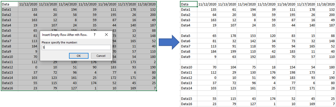
![]() Insert Footer: Allows the User to apply a Custom Center Section Footer on all worksheets. If it contains the words confidentiality, secret or classified, the text colour is set to Red.
Insert Footer: Allows the User to apply a Custom Center Section Footer on all worksheets. If it contains the words confidentiality, secret or classified, the text colour is set to Red.
![]() Insert Table of Contents: Inserts a new sheet with hyperlinks to each sheet and an image of the 1st 5 rows and 11 columns of the sheets.
Insert Table of Contents: Inserts a new sheet with hyperlinks to each sheet and an image of the 1st 5 rows and 11 columns of the sheets.
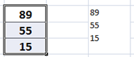
![]() Split Text Down: For a cell containing carriage returns, Splits the text into cells in newly inserted rows below.
Split Text Down: For a cell containing carriage returns, Splits the text into cells in newly inserted rows below.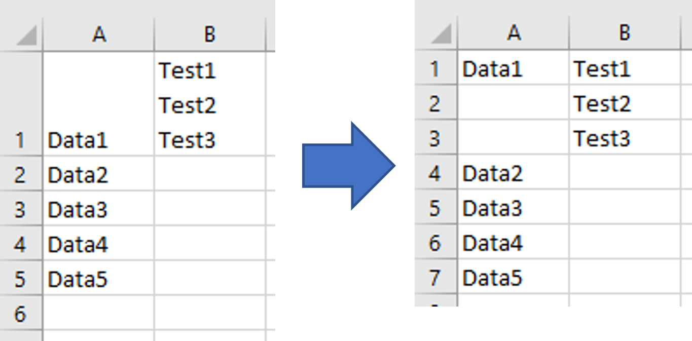
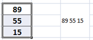
![]() Split Text Right: For a cell containing carriage returns, Splits the text into cells in newly inserted columns to the right.
Split Text Right: For a cell containing carriage returns, Splits the text into cells in newly inserted columns to the right.
![]() Join, Merge and Wrap: Based on the selected cells, merges the cells and text within the cells inserting a carriage return between cell entries.
Join, Merge and Wrap: Based on the selected cells, merges the cells and text within the cells inserting a carriage return between cell entries.
![]() Join and Merge: Based on the selected cells, merges the cells and text within the cells.
Join and Merge: Based on the selected cells, merges the cells and text within the cells.
![]() Make Cells Square: Sets the cells in a worksheet to be square based on a row height of 15.
Make Cells Square: Sets the cells in a worksheet to be square based on a row height of 15.
![]() Merge Same: Merges cells in a column with the same value in the selected range. Works best with values not formulas. Use the Formula to Value tool in Misc Tools to convert formulas to values.
Merge Same: Merges cells in a column with the same value in the selected range. Works best with values not formulas. Use the Formula to Value tool in Misc Tools to convert formulas to values.

![]() Reset Used Range: Resets the active area in the current worksheet. Typically used after many rows of data have been deleted.
Reset Used Range: Resets the active area in the current worksheet. Typically used after many rows of data have been deleted.
 Forms
Forms
![]() Add Month Calendar: Inserts a new Sheet with an editable Calendar based on user input.
Add Month Calendar: Inserts a new Sheet with an editable Calendar based on user input.

![]() Add Problem Tracking Sheet: Inserts a new Sheet formatted as a basic Problem Tracking sheet. There are associated PowerPoint functions to create a Problem Tracking chart. The column headings are set up as named ranges allowing the text to be modified and the columns rearranged while maintaining the PowerPoint output to remain the same.
Add Problem Tracking Sheet: Inserts a new Sheet formatted as a basic Problem Tracking sheet. There are associated PowerPoint functions to create a Problem Tracking chart. The column headings are set up as named ranges allowing the text to be modified and the columns rearranged while maintaining the PowerPoint output to remain the same.

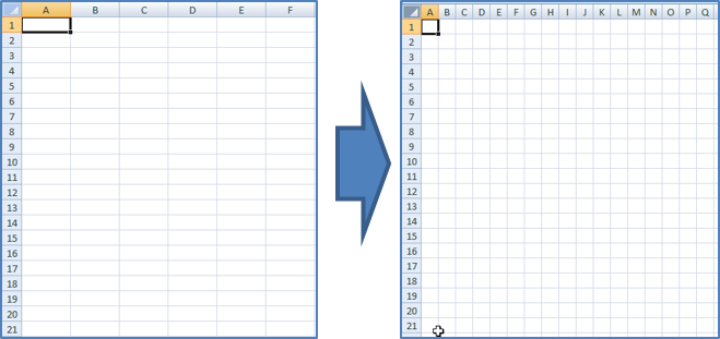
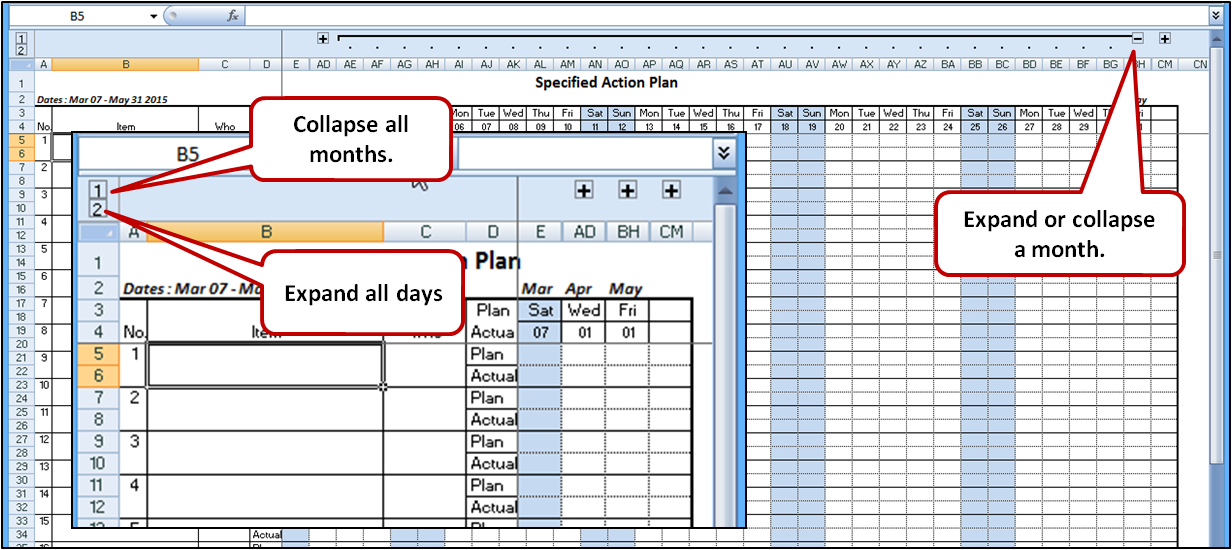
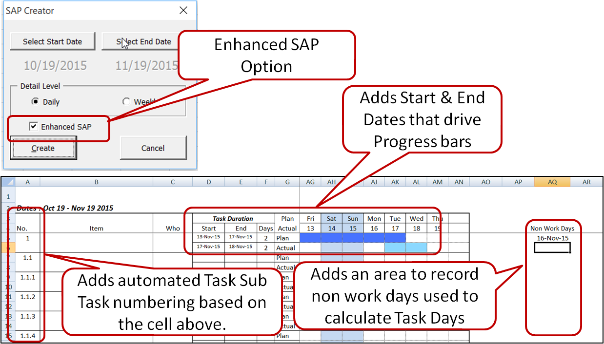
![]() Add SAP: Inserts a new Sheet with an editable SAP based on user input. The user selects the Start and End dates and can choose between Daily and Weekly SAPs. For Weekly SAPS, weeks start on Mondays and the first week contains the user selected Start date. The default Start Date is the current date. The default End Date is 31 days later.
Add SAP: Inserts a new Sheet with an editable SAP based on user input. The user selects the Start and End dates and can choose between Daily and Weekly SAPs. For Weekly SAPS, weeks start on Mondays and the first week contains the user selected Start date. The default Start Date is the current date. The default End Date is 31 days later.

Feature updated to allow Daily or Weekly SAPs to be collapsed to display by month.
Feature updated to include Start and End Dates that drive Taskbars.
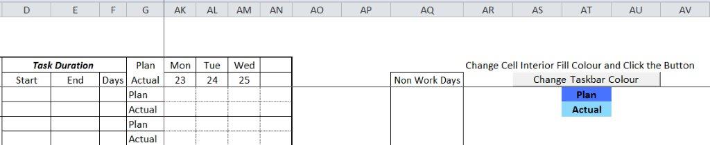
Feature updated to allow users to change the Taskbar colours by changing the interior fill colour of 2 cells and clicking an update button.
Feature updated to allow users to include or exclude Sat Sun & Holidays in Days calculation.

The Add Shapes Section contains a number of utilities to add Clip Art and custom shapes. (video overview)
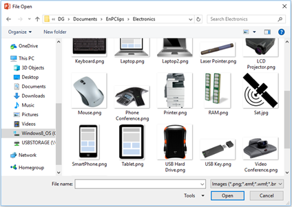
![]() EnP Clips:Allows the user to insert an images and Clip Art found in specific folders located in user’s Documents\EnPClips folder. The user can add their own “favourite” images to the exiting folder(s) or add their own folder(s) to the user’s Documents\EnPClips folder. EnP Tools comes with a few examples to get you started.
EnP Clips:Allows the user to insert an images and Clip Art found in specific folders located in user’s Documents\EnPClips folder. The user can add their own “favourite” images to the exiting folder(s) or add their own folder(s) to the user’s Documents\EnPClips folder. EnP Tools comes with a few examples to get you started.
Examples:
The Custom Shapes menu has 3 specialized functions to add different shapes.
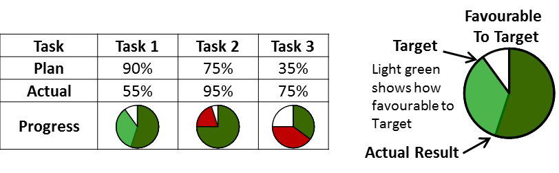
![]() Progress Pies can be used to report on the progress of a task or activity.
Progress Pies can be used to report on the progress of a task or activity.
Greater is Favourable: From the selected range of Actuals, returns circular representations of task completion rates based on Plan vs Actual where Actual greater than Plan is favourable. The Progress Pies are pasted to the right or below the selected cells. Targets must be in the adjacent cells above or to the left of the Actuals – both to be entered as percentages.

Less is Favourable: From the selected range of Actuals, returns circular representations of task completion rates based on Plan vs Actual where Actual less than Plan is favourable. The Progress Pies are pasted to the right or below the selected cells. Targets must be in the adjacent cells above or to the left of the Actuals – both to be entered as percentages.
 Progress Pie Black: From the selected range of Actuals, returns black circular representations of task completion rates. The Progress Pies are pasted to the right or below the selected cells. The Actuals are to be entered as percentages.
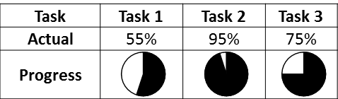
NOTE: Functions will work with horizontal or vertical ranges. Single cell selections will place the Progress Pie to the right.
Misc Shapes
![]() Add Rectangle: Adds a red Rectangle around the selected cells that can be used to indicate a focus area.
Add Rectangle: Adds a red Rectangle around the selected cells that can be used to indicate a focus area.![]()
![]() Add Time Line: Adds or deletes a grouped shape – reverse “S” time line graphic.
Add Time Line: Adds or deletes a grouped shape – reverse “S” time line graphic.

![]() Rounded Rectangle: Adds a red Rounded Rectangle that can be used to indicate focus areas.
Rounded Rectangle: Adds a red Rounded Rectangle that can be used to indicate focus areas.
![]()
![]() Callout: Adds a red Rounded Callout that can be used to indicate focus areas.
Callout: Adds a red Rounded Callout that can be used to indicate focus areas.

![]() Approval Box: Adds a Approval sign off box at the current cell location. The first blank cells are intended for the names and the second row for the dates.
Approval Box: Adds a Approval sign off box at the current cell location. The first blank cells are intended for the names and the second row for the dates.
![]()
![]() Cross Over Connector – Horizontal
Cross Over Connector – Horizontal
![]() Cross Over Connector – Vertical: Adds a set of connectors that can be used in flow charts for cross overs. It adds 3 joined MS Office shapes – a straight connector, an arc and a straight line arrow. The straight connector and arrow are meant to be connected to the flow chart symbols. The arc is best moved with the keyboard arrow keys – up and down, side to side. The same connectors are available in Excel.
Cross Over Connector – Vertical: Adds a set of connectors that can be used in flow charts for cross overs. It adds 3 joined MS Office shapes – a straight connector, an arc and a straight line arrow. The straight connector and arrow are meant to be connected to the flow chart symbols. The arc is best moved with the keyboard arrow keys – up and down, side to side. The same connectors are available in Excel.

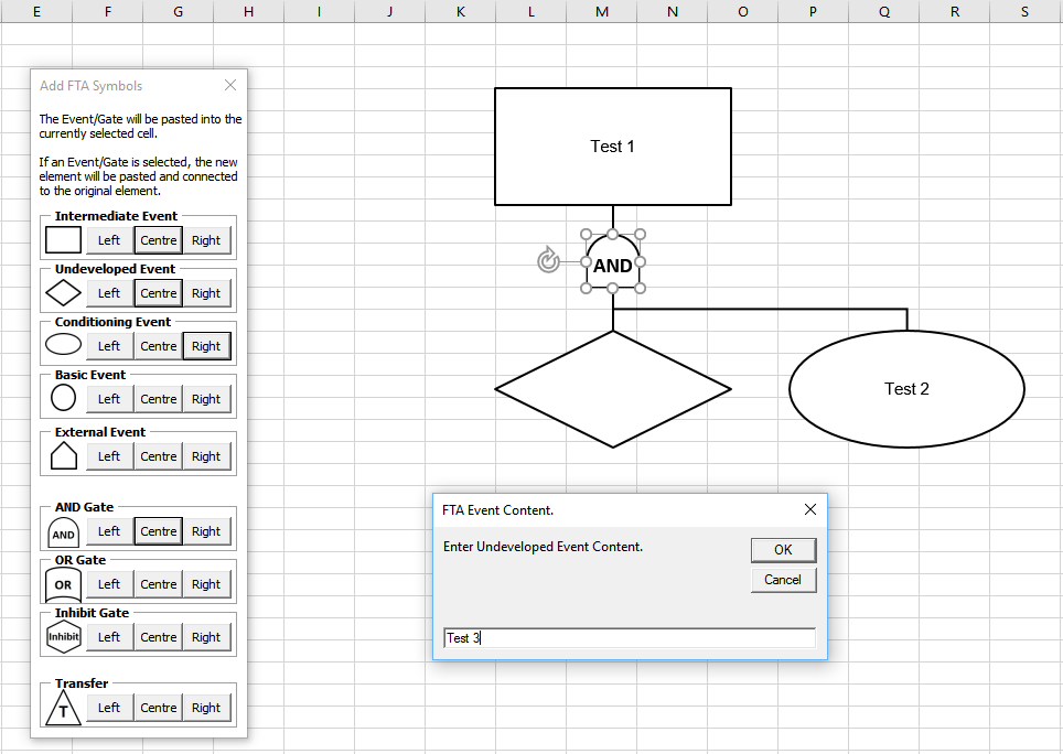
![]() FTA Symbols: Displays a form from which the User can add symbols to build an FTA chart. The Event/Gate will be pasted into the currently selected cell. If an Event/Gate is selected, the new element will be pasted and connected to the original element.
FTA Symbols: Displays a form from which the User can add symbols to build an FTA chart. The Event/Gate will be pasted into the currently selected cell. If an Event/Gate is selected, the new element will be pasted and connected to the original element.
 Yamataka Tools: A set of tools to help build Yamataka / Waterfall charts from simple rectangles:
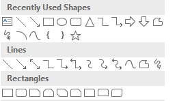
![]() Add Shapes and Connectors: Displays the MS Office Autoshapes gallery. Right clicking on a shape and selecting “Lock Drawing Mode” will allow the User to draw multiple versions of the selected shape.
Add Shapes and Connectors: Displays the MS Office Autoshapes gallery. Right clicking on a shape and selecting “Lock Drawing Mode” will allow the User to draw multiple versions of the selected shape.
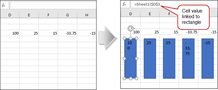
![]() Add Linked Rectangles: Adds rectangles with text linked to the cell values of the selected range. If the range is horizontal, the rectangles will be placed beneath the selected range as below. If the range is vertical, the rectangles are placed to the right of the range. These rectangles can be used to start the Yamataka building process.
Add Linked Rectangles: Adds rectangles with text linked to the cell values of the selected range. If the range is horizontal, the rectangles will be placed beneath the selected range as below. If the range is vertical, the rectangles are placed to the right of the range. These rectangles can be used to start the Yamataka building process.
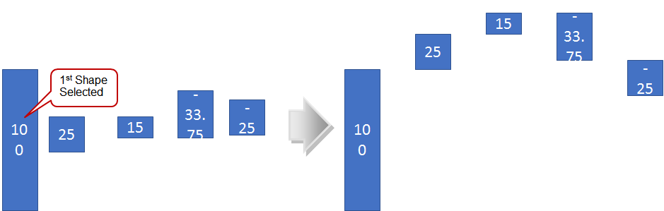
![]() Size Proportional: Proportionately sets the height of the selected shapes in relation to the height of the first selected shape and its text while setting the width to be the same as the first shape.
Size Proportional: Proportionately sets the height of the selected shapes in relation to the height of the first selected shape and its text while setting the width to be the same as the first shape.

![]() Cascade: Arranges the selected shapes (beginning with the first selected shape) into the basic cascade arrangement of a Yamataka or Waterfall chart. It takes into account whether or not the values in the rectangles are positive or negative and aligns the shapes appropriately. It also horizontally spaces the shapes based on the width of the first shape.
Cascade: Arranges the selected shapes (beginning with the first selected shape) into the basic cascade arrangement of a Yamataka or Waterfall chart. It takes into account whether or not the values in the rectangles are positive or negative and aligns the shapes appropriately. It also horizontally spaces the shapes based on the width of the first shape.
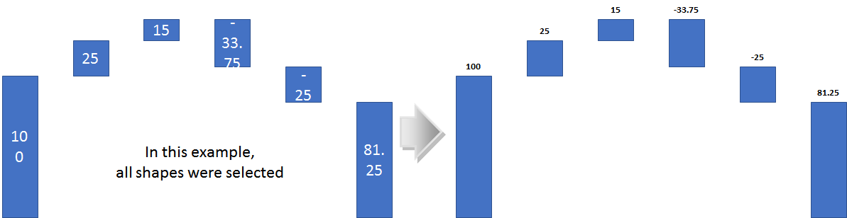
![]() Add Summary Bar: Creates a rectangle with the sum of the values of the selected shapes as it’s text value, sets the height and width relative to the 1st selected shape then aligns it’s bottom to that shape.
Add Summary Bar: Creates a rectangle with the sum of the values of the selected shapes as it’s text value, sets the height and width relative to the 1st selected shape then aligns it’s bottom to that shape.
![]() Move Text Above: Creates a text box above the selected rectangle with the rectangle’s text and then deletes the original text in the rectangle.
Move Text Above: Creates a text box above the selected rectangle with the rectangle’s text and then deletes the original text in the rectangle.
![]() Erase Shapes: Erases All Shapes (pictures, graphs, textboxes, autoshapes, etc…) in the selected range.
Erase Shapes: Erases All Shapes (pictures, graphs, textboxes, autoshapes, etc…) in the selected range.
Size and Arrange Shapes: A number of functions to size and arrange selected shapes. (video overview)
![]() Same Size: Adjusts the size of the selected Shapes to the size of the last selected Shape.
Same Size: Adjusts the size of the selected Shapes to the size of the last selected Shape.

![]() Same Height: Adjusts the height of the selected Shapes to the height of the last selected Shape.
Same Height: Adjusts the height of the selected Shapes to the height of the last selected Shape.

![]() Same Width: Adjusts the width of the selected Shapes to the width of the last selected Shape.
Same Width: Adjusts the width of the selected Shapes to the width of the last selected Shape.

![]() Bottom Edge Align: Aligns the top edge of the selected Shapes to the bottom edge of the last selected Shape.
Bottom Edge Align: Aligns the top edge of the selected Shapes to the bottom edge of the last selected Shape.

![]() Top Edge Align: Aligns the bottom edge of the selected Shapes to the top edge of the last selected shape.
Top Edge Align: Aligns the bottom edge of the selected Shapes to the top edge of the last selected shape.

![]() Right Edge Align: Aligns the left edge of the selected Shapes to the right edge of the last selected Shape.
Right Edge Align: Aligns the left edge of the selected Shapes to the right edge of the last selected Shape.

![]() Left Edge Align: Aligns the right edge of the selected Shapes to the left edge of the last selected Shape.
Left Edge Align: Aligns the right edge of the selected Shapes to the left edge of the last selected Shape.

![]() Spacing Vertical: Distributes the Selected Shapes, in order of Selection, below the Last Selected Shape by the number of Points entered.
Spacing Vertical: Distributes the Selected Shapes, in order of Selection, below the Last Selected Shape by the number of Points entered.
![]() Spacing Horizontal: Distributes the Selected Shapes, in order of Selection, to the right of the Last Selected Shape by the number of Points entered.
Spacing Horizontal: Distributes the Selected Shapes, in order of Selection, to the right of the Last Selected Shape by the number of Points entered.
Misc
![]() Grow And Shrink: Expand and Contract the Selected Shapes along the non-rotated height and width axes.
Grow And Shrink: Expand and Contract the Selected Shapes along the non-rotated height and width axes.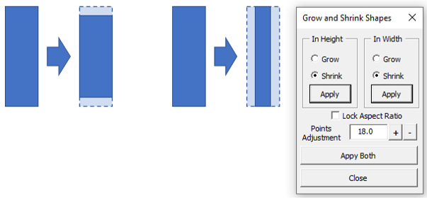
![]() Line Snap: Makes the Selected Lines or Connectors horizontal or vertical based on their slope.
Line Snap: Makes the Selected Lines or Connectors horizontal or vertical based on their slope.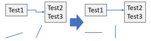
![]() Size Get: Gets the size of the selected shape. To be used in conjunction with the Size Set feature to match sizes.
Size Get: Gets the size of the selected shape. To be used in conjunction with the Size Set feature to match sizes.
![]() Size Set: Sets the size of the selected shape. To be used in conjunction with the Size Get feature to match sizes.
Size Set: Sets the size of the selected shape. To be used in conjunction with the Size Get feature to match sizes.
![]() Stretch Down: Stretches the bottom edge of the first of two selected shapes to the top edge of the second shape.
Stretch Down: Stretches the bottom edge of the first of two selected shapes to the top edge of the second shape.
![]() Stretch Up: Stretches the top edge of the first of two selected shapes to the bottom edge of the second shape.
Stretch Up: Stretches the top edge of the first of two selected shapes to the bottom edge of the second shape.
![]() Stretch Up: Stretches the top edge of the first of two selected shapes to the bottom edge of the second shape.
Stretch Up: Stretches the top edge of the first of two selected shapes to the bottom edge of the second shape.
![]() Stretch Up: Stretches the top edge of the first of two selected shapes to the bottom edge of the second shape.
Stretch Up: Stretches the top edge of the first of two selected shapes to the bottom edge of the second shape.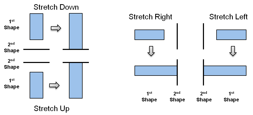
![]() Switch: Switches the Positions of the 2 Selected Shapes.
Switch: Switches the Positions of the 2 Selected Shapes.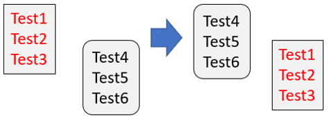
 PowerPoint: Macros providing functionality between Excel and PowerPoint (video overview)
![]() Range as Picture to PPT – Fit Height: Copies the selected range, pastes it as a picture into a new Slide resized if its Height is greater than Slide Height.
Range as Picture to PPT – Fit Height: Copies the selected range, pastes it as a picture into a new Slide resized if its Height is greater than Slide Height.
![]() Range as Picture to PPT – Fit Width: Copies the selected range, pastes it as a picture into a new Slide resized if its Width is greater than Slide Width.
Range as Picture to PPT – Fit Width: Copies the selected range, pastes it as a picture into a new Slide resized if its Width is greater than Slide Width.

![]() Range as Picture to PPT – Fit Slide: Copies the selected range, pastes it as a picture into a new Slide resized if required based on its Height or Width whichever fits best.
Range as Picture to PPT – Fit Slide: Copies the selected range, pastes it as a picture into a new Slide resized if required based on its Height or Width whichever fits best.
![]() Embed Selection on Slide: Copies the selected range, embeds it as an Excel file into a new Slide resized if required based on its Height or Width whichever fits best.
Embed Selection on Slide: Copies the selected range, embeds it as an Excel file into a new Slide resized if required based on its Height or Width whichever fits best.
![]() Chart as Picture to PPT – Fit Slide: Copies the selected Chart, pastes it as a picture into a new Slide resized if required based on its Height or Width whichever fits best.
Chart as Picture to PPT – Fit Slide: Copies the selected Chart, pastes it as a picture into a new Slide resized if required based on its Height or Width whichever fits best.
![]() Embed Chart on Slide: Copies the selected Chart, embeds it as an Excel file into a new Slide resized if required based on its Height or Width whichever fits best.
Embed Chart on Slide: Copies the selected Chart, embeds it as an Excel file into a new Slide resized if required based on its Height or Width whichever fits best.
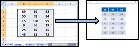
![]() Selected Range Insert Table: Creates a Slide with a Table populated from the selected range but does not fit Table to Slide. Slow based on range size.
Selected Range Insert Table: Creates a Slide with a Table populated from the selected range but does not fit Table to Slide. Slow based on range size.
Problem Tracking Charts
The functions provided in this section provide 3 ways to create PowerPoint slides from a row in a specially formatted Excel sheet. Included are 2 mechanisms to allow users to format a sheet to work with the create functions.
The simplest way to use the first 2 functions is to add the specially formatted sheet via the Worksheet Tools – Forms function: Add Problem Tracking Sheet. This function provides a basic sheet that users can immediately start using without employing the “Prep” functions described further down. Each cell in the Title row is named (e.g. PT_01) in order to determine which content goes where in the PowerPoint slide. Note: moving the columns in the spreadsheet is possible; however, the PowerPoint layout is fixed.
Create a Problem Tracking Chart: From a properly formatted sheet, this feature will copy information from the current row and create a specifically formatted PowerPoint presentation. The user will be prompted to save the presentation. A suggested file name is derived from 3 columns containing the named ranges – PT_01, PT_02 & PT_03; however, the user can choose a different name or not to save the file at that time. If the presentation is saved, a hyper-link will be created to the saved file on the exported row. The hyper-link will be attached to the value that resides in the same column as the named range PT_01 in the exported row. A single Image can be transferred but its location on the Excel sheet but in the same column as the named range PT_07. This column on the sheet created by the Worksheet Tools – Forms function: Add Problem Tracking Sheet function is cleverly titled “Image”. If no images are required, the cell can be used for additional text.

Create a Problem Tracking Chart with Image Annotation: Performs as above with one exception regarding the image. Using this function transfers the contents of the cell – any image, call-out, shape, etc… as a single image. Any annotation on the image from the Excel file will transfer to the presentation; however, it will not be editable.
Create a Problem Tracking Chart from Template: Creates a PowerPoint slide from the current row from a EnP Tools problem tracking sheet using a user created template. The Excel sheet must be prepared using the tool “Prep PTC Sheet for PowerPoint Template” (see below). Also, a template file “Custom_EnP_PTC.pptx” must be in the Documents folder. The template file can be created using EnP Tools for PowerPoint under Utilities – Misc Tools: Convert to PTC Template. Images can be in any of the “mapped” Excel columns. The combination of the PowerPoint & Excel functions provides a significant level of flexibility in creating PowerPoint summary slides from Excel. Once a template is created, copying the Excel data to the template is faster than the functions above due to the fact that no rectangles are drawn and formatted.
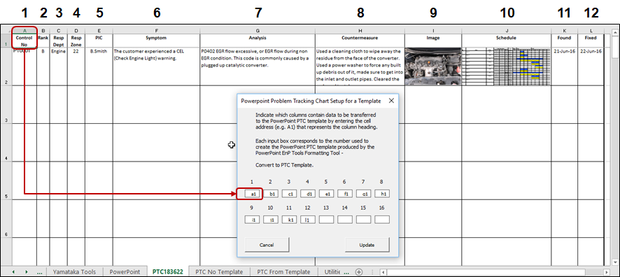
Prep PTC Sheet for PowerPoint: Allows the user to select columns to be exported to a PowerPoint PTC slide. Opens a form to map specific column cells to the PowerPoint Problem Tracking Chart. This allows any worksheet to be used as a source to create a PowerPoint Problem Tracking Chart. The mapped cells are set up as named ranges allowing the text to be modified and the columns rearranged while maintaining the PowerPoint output to remain the same.

Prep PTC Sheet for PowerPoint Template: Allows the user to select up to 16 columns to be exported to a PowerPoint PTC slide utilizing the user created “Custom_EnP_PTC.pptx” template in the Documents folder. The template file can be created using EnP Tools for PowerPoint under Utilities – Misc Tools: Convert to PTC Template. Images can be in any of the “mapped” Excel columns.
 Utilities: A number of misc tools including Picture Insert Tools. (video overview)
There are 2 categories:
1) Picture Insert Tools – utilities that assist in the insertion and placement of images and shapes.
2) Misc Tools
 Picture Insert Tools – utilities that assist in the insertion and placement of images and shapes.
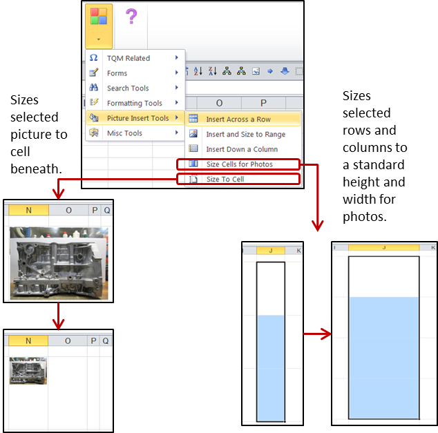
![]() Insert Across a Row: Allows users to multi-select pictures to insert across a row of cells. Upon insert the pictures are sized to the cells.
Insert Across a Row: Allows users to multi-select pictures to insert across a row of cells. Upon insert the pictures are sized to the cells.

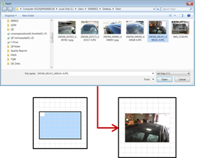
![]() Insert and Size to Range: Allows users to insert and resize a picture to a selected range.
Insert and Size to Range: Allows users to insert and resize a picture to a selected range.
![]() Insert Down a Column: Allows users to multi-select pictures to insert down a column of cells. Upon insert the pictures are sized to the cells.
Insert Down a Column: Allows users to multi-select pictures to insert down a column of cells. Upon insert the pictures are sized to the cells.
![]() Size Cell for Photos: Sizes selected rows and columns to a standard height and width photos.
Size Cell for Photos: Sizes selected rows and columns to a standard height and width photos.
![]() Size To Cell: Sizes selected picture to cell beneath.
Size To Cell: Sizes selected picture to cell beneath.
 Misc Tools
![]() Add Custom List: From the Selected Range, creates a Custom List that can be used with AutoFill. Once you create a custom list, it is added to your computer registry, so that it is available for use in other workbooks. However, if you open the workbook on another computer or server, you do not see the custom list.
Add Custom List: From the Selected Range, creates a Custom List that can be used with AutoFill. Once you create a custom list, it is added to your computer registry, so that it is available for use in other workbooks. However, if you open the workbook on another computer or server, you do not see the custom list.
![]() Add Random Data: Tools to add random data to Selected cells.
Add Random Data: Tools to add random data to Selected cells.
![]() Add Random Numbers: Adds random numbers between 0 and 100 to the selected range.
Add Random Numbers: Adds random numbers between 0 and 100 to the selected range.

![]() Add Random Word: Add a random word from the Lorem Ipsum text to the selected range.
Add Random Word: Add a random word from the Lorem Ipsum text to the selected range.
![]() Add Sample Chart Data: Adds a block of random numbers with row and column headings to the selected Range. The selected range must be at least 3×3. The resulting sample data will have dates across the top starting from the current date and row labels – Data1, Data2, etc….
Add Sample Chart Data: Adds a block of random numbers with row and column headings to the selected Range. The selected range must be at least 3×3. The resulting sample data will have dates across the top starting from the current date and row labels – Data1, Data2, etc….
![]() Break Links: Converts all formulas linked to other Microsoft Excel sources or OLE sources to values. Example: Workbook Test1.xlsx has a formula linked to Workbook Test2.xlsx “=[Test2.xlsx]Sheet1!$A$1” whose value is 250. This function will convert the formula in Test1.xlsx to the value 250. This also works with charts. This is useful when the sources are no longer available.
Break Links: Converts all formulas linked to other Microsoft Excel sources or OLE sources to values. Example: Workbook Test1.xlsx has a formula linked to Workbook Test2.xlsx “=[Test2.xlsx]Sheet1!$A$1” whose value is 250. This function will convert the formula in Test1.xlsx to the value 250. This also works with charts. This is useful when the sources are no longer available.
![]() Copy Row by Colour: From the Selection, copies rows to a new sheet if the rows have any colour filled cells not Conditionally Formatted.
Copy Row by Colour: From the Selection, copies rows to a new sheet if the rows have any colour filled cells not Conditionally Formatted.
![]() Create Compressed Copy: Creates a compressed copy of the active workbook in C:Temp. XLSX and XLSM files are “zipped” XML files. This process unzips and then re-zips the Excel file to gain some additional compression. This is can reduce large data files but does not have a significant impact to files containing images. “Compressed xx-xx-xx” is appended to the compressed copy file name. Below demonstrates the amount of compression gained as compared to zipping in Windows Explorer.
Create Compressed Copy: Creates a compressed copy of the active workbook in C:Temp. XLSX and XLSM files are “zipped” XML files. This process unzips and then re-zips the Excel file to gain some additional compression. This is can reduce large data files but does not have a significant impact to files containing images. “Compressed xx-xx-xx” is appended to the compressed copy file name. Below demonstrates the amount of compression gained as compared to zipping in Windows Explorer.

![]() Create File List: From the selected folder, creates a file list on a new worksheet. Note: the function is not recursive i.e. sub-folders are ignored. The Open hyperlink opens the file.
Create File List: From the selected folder, creates a file list on a new worksheet. Note: the function is not recursive i.e. sub-folders are ignored. The Open hyperlink opens the file.
![]() Delete Names: Delete all named ranges in the workbook (except hidden names). This is useful when the named ranges are causing issues with copying worksheets within the workbook i.e. warning dialogs are displayed. Note: Deleting Named Ranges with Japanese Names from the Name Manager on English machines may not actually delete the Name from the workbook only from the Name Manager. This function will delete the Japanese Name as well.
Delete Names: Delete all named ranges in the workbook (except hidden names). This is useful when the named ranges are causing issues with copying worksheets within the workbook i.e. warning dialogs are displayed. Note: Deleting Named Ranges with Japanese Names from the Name Manager on English machines may not actually delete the Name from the workbook only from the Name Manager. This function will delete the Japanese Name as well.
![]() Extract Tools: Tools to extract and save Media and Notes from Workbooks.
Extract Tools: Tools to extract and save Media and Notes from Workbooks.
![]() Extract Media to Folders: Extracts copies of the embedded image files and places them in folders. Windows Explorer is opened to the targeted folder.
Extract Media to Folders: Extracts copies of the embedded image files and places them in folders. Windows Explorer is opened to the targeted folder.
![]() Extract Notes: Combines the Workbook Notes as a text file in the Workbook folder. Info extracted – Sheet Name, Cell Address, Cell Value and Note. The text file is placed in the same folder as the Workbook.
Extract Notes: Combines the Workbook Notes as a text file in the Workbook folder. Info extracted – Sheet Name, Cell Address, Cell Value and Note. The text file is placed in the same folder as the Workbook.
e.g. TestFile – Notes.txt
![]() Extract To EnP Clips: Extracts the Selected Shapes to a folder with the Workbook name in the EnPClips – Shape Extracts folder. The extracted shapes can be saved as BMP, GIF, JPG or PNG files.
Extract To EnP Clips: Extracts the Selected Shapes to a folder with the Workbook name in the EnPClips – Shape Extracts folder. The extracted shapes can be saved as BMP, GIF, JPG or PNG files.
Notes:
1) The following Shape Types are not supported – msoShapeTypeMixed, msoComment, msoEmbeddedOLEObject, msoLinkedOLEObject, msoOLEControlObject, msoPlaceholder, msoTextEffect, msoMedia, msoScriptAnchor, msoCanvas, msoDiagram, msoInk, msoIgxGraphic, msoWebVideo, msoContentApp, msoGraphic, msoLinkedGraphic, mso3DModel, msoLinked3DModel
2) Checking the “Do not compress images in file” option provides maximum picture quality but may result in very large file sizes.
![]() Text To Cells: Places the Selected Shape’s Text in separate cells starting in the cell beneath the Shape’s top left corner and deletes the Shape.
Text To Cells: Places the Selected Shape’s Text in separate cells starting in the cell beneath the Shape’s top left corner and deletes the Shape.
![]() Formula to Value: Converts formulas to values in the current selection.
Formula to Value: Converts formulas to values in the current selection.
![]() Password Tools: Tools to Set, Reset and Store Password Information. If the Workbook is opened Read-Only, the Set Passwords section is disabled as you cannot change the passwords in a Read-Only state. When the form is opened, the current Windows user name is displayed in the textboxes as a password suggestion. The User can type their own password or click the Generate Password button to generate a random 8 character password. Clicking the Clear button will delete the text in the corresponding textbox. Clicking the Set Password button at this time will Reset the password to nothing. If there are characters displayed in the textbox, clicking a Set Password button will set the appropriate password, save the workbook and add the workbook location, name , date, password type and password to the Password Record. View Password Records – opens a text file listing the files and passwords set by EnP Tools. This file is located in EnP Tools folder in the User’s Documents folder – EnP_PSWs.txt
Password Tools: Tools to Set, Reset and Store Password Information. If the Workbook is opened Read-Only, the Set Passwords section is disabled as you cannot change the passwords in a Read-Only state. When the form is opened, the current Windows user name is displayed in the textboxes as a password suggestion. The User can type their own password or click the Generate Password button to generate a random 8 character password. Clicking the Clear button will delete the text in the corresponding textbox. Clicking the Set Password button at this time will Reset the password to nothing. If there are characters displayed in the textbox, clicking a Set Password button will set the appropriate password, save the workbook and add the workbook location, name , date, password type and password to the Password Record. View Password Records – opens a text file listing the files and passwords set by EnP Tools. This file is located in EnP Tools folder in the User’s Documents folder – EnP_PSWs.txt
Note: The password types are native to PowerPoint. Setting the Open password encrypts the workbook while setting a Modify password does not. It is not a security feature as it is only meant to protect from unintentional editing.
Set Protection: Lists the worksheets available in the workbook. Upon opening, any Password protected sheets are selected. The buttons allow the user to select specific sheets based on the Protection status. Sheets can be multi-selected using the Shift ot Control keys. The textbox is used to provide Password information for both protecting and unprotecting worksheets. If the textbox is empty, the sheets are protected with no Password when the Protect button is clicked. The “Allow Users to” options set the protection criteria. Clicking the Protect button protects the selected sheets and stores the Protection information and password in the EnP_PSWs file. If the password in the textbox does not match and existing password for a protected sheet, that sheet is skipped until the correct password is provided. The Unprotect button works similarly.
Create Protection Sheet Status: Creates a new sheet that summarizes the protection status of each sheet in the workbook.
Remove: Allows the User to remove the Workbook and Worksheet(s) passwords from a closed xlsx file. The User selects a file to be processed. Upon completion an unprotected version of the will be created in the same folder as the source file. The new file will have “Unprotected” appended to the source file name. Finally, Windows File Explorer will be opened to the appropriate folder. Note: Files other than XLSX or require a Password to Open will not be processed.
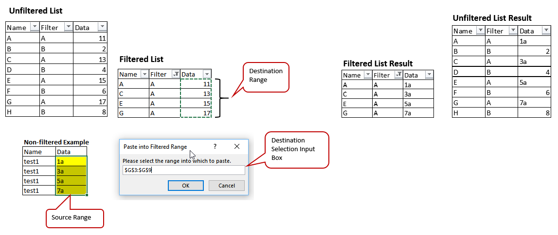
![]() Paste To Filtered Range: Copies the currently select range within a single column and pastes it to a user selected single column range while skipping any hidden rows. Typically used on filtered ranges. The source range can be a filtered list as well.
Paste To Filtered Range: Copies the currently select range within a single column and pastes it to a user selected single column range while skipping any hidden rows. Typically used on filtered ranges. The source range can be a filtered list as well.
![]() Personal Tab Creator: Open a workbook which includes a Personal Tab on the Ribbon that can be used to run up to 10 user created macros.
Personal Tab Creator: Open a workbook which includes a Personal Tab on the Ribbon that can be used to run up to 10 user created macros.

Basic Steps
- Display the Visual Basic Editor (VBE)
– key Alt + F11. - Add your own code to the starter macros provided in the Custom_Macro_Module . DO NOT change the names of the macros!
- Optional but recommended – delete this sheet
- Save the presentation (you can change the Name but make sure you save it as a Macro-Enable file (*.xlsm or *.xltm).
Optional: You can change:
- The name of the Tab (from Personal Tab)
- The name of the Group (from Personal Macros)
- The name of the Button (from Macro 1, Macro 2, etc…)
- The additional info for the macros in the “supertip”
If you do not need all 10 Buttons, you can hide them by setting the Visible Constant to False.
To create an Excel Add-In:
After completing the steps above, use the SAVE AS option to save the presentation as a Excel Add-in (*.xlam). Save it to the default folder provided.
To Install the Add-in (.xlam) File
- Go To File, then Options
- Select Add-Ins
- Select Excel Add-Ins from the “Manage” drop-down and click Go
- Check the box beside the newly created Add-in and Click OK. Your Personal Tab should now be available each time you open Excel. Note: if you didn’t see your file name, select Browse, go to where you saved the file, double click it and Click OK.
![]() Shapes Stats: Provides the dimensions and position of the selected shape in both points and inches. A “point” is a unit of measurement that is equal to 1/72 of an inch.
Shapes Stats: Provides the dimensions and position of the selected shape in both points and inches. A “point” is a unit of measurement that is equal to 1/72 of an inch.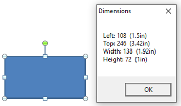
![]() Show Calculator: Opens the MS Calculator.
Show Calculator: Opens the MS Calculator.
![]() Sum Selected: Sums the Selected Cells and copies the result to the clipboard. Also available as a right click menu item.
Sum Selected: Sums the Selected Cells and copies the result to the clipboard. Also available as a right click menu item.
![]() System Info: Displays IP Configuration and WMI Information.
System Info: Displays IP Configuration and WMI Information.
![]() IP Config Info: Adds a new sheet listing all current TCP IP network configuration values.
IP Config Info: Adds a new sheet listing all current TCP IP network configuration values.
![]() WMI Info: Adds a new sheet listing all current TCP IP network configuration values.
WMI Info: Adds a new sheet listing all current TCP IP network configuration values.
![]() Toggle Lorem Ipsum: Toggles the selected Shapes’ text between a Lorem Ipsum string and the original text. A simple way to temporarily “hide” confidential information for printing.
Toggle Lorem Ipsum: Toggles the selected Shapes’ text between a Lorem Ipsum string and the original text. A simple way to temporarily “hide” confidential information for printing.
Functions

A number of custom functions that are also available to through the Excel Insert Function command and listed in an EnP Tools category.
EnP Function Categories
Date Info Logical Math Text Misc
Note: Workbooks with EnP Tool functions authored by other Users using EnP Tools will display the following dialog prior to resetting the Functions’ add-in path. The dialog can be dismissed.

If the Functions display #NAME! errors and the User’s complete path to the location of the add-in is shown in each formula, clicking the Reset button on the EnP Tools Custom Functions dialog will fix the issue.

Date Functions:
BetweenDays(Start_Date As Date, End_Date As Date) As Long
Returns the number of Days between to Dates.
Start_Date: The Start Date
End_Date: The End Date
BetweenMonths(Start_Date As Date, End_Date As Date) As Long
Returns the number of Days between to Dates.
Start_Date: The Start Date
End_Date: The End Date
BetweenWeeks(Start_Date As Date, End_Date As Date) As Long
Returns the number of Weeks between to Dates.
Start_Date: The Start Date
End_Date: The End Date
BetweenYears(Start_Date As Date, End_Date As Date) As Long
Returns the number of Years between to Dates. When comparing December 31 to January 1 of the immediately succeeding year, returns 1 even though only a day has elapsed.
Start_Date: The Start Date
End_Date: The End Date
H_EmancipationDay(Yr As Integer) As String
Returns the date of the Canadian Emancipation Day Holiday.
Yr: The Year as an Integer.
H_FamilyDay(Yr As Integer) As String
Returns the date of the Canadian Family Holiday.
Yr: The Year as an Integer.
H_GoodFriEaster(YYYY As Long, Optional GoodFriday As Boolean = True) As String
Returns the date of Good Friday or Easter. Works for years 1900 to 2368.
YYYY: The Year as an Integer.
GoodFriday: (Optional) True: Good Friday (default). False: Easter.
H_LabourDay(Yr As Integer) As String
Returns the date of the Labour Day Holiday.
Yr: The Year as an Integer.
H_ThanksgivingCA(Yr As Integer) As String
Returns the date of the Canadian Thanksgiving Holiday.
Yr: The Year as an Integer.
H_ThanksgivingUS(Yr As Integer) As String
Returns the date of the US Thanksgiving Holiday.
Yr: The Year as an Integer.
H_VictoriaDay(Yr As Integer) As String
Returns the date of the Canadian Victoria Day Holiday.
Yr: The Year as an Integer.
Julian2StdDate(JDate As Variant)
Converts a Julian Date to a Standard Date.
JDate: The Julian Date or Cell containing a Julian Date to be converted.
NthDayOfWeek(N As Variant, DoW As Variant, Mo As Variant, Yr As Integer) As String
NthDayOfWeek( 3,2,1,2021) or NthDayOfWeek(“3rd”,”Mon”,”Jan”, 2021) returns the date for the 3rd Monday in January 2021.
N: Iteration. Valid parameters for 3rd week: 3 ,”3rd” or “Third” (case insensitive).
DoW: Day of Week. Valid parameters for Monday: 2 ,”Mon”, “Mon.” or “Monday” (case insensitive). Saturday = 0.
Mo: Month. Valid parameters for January: 1 ,”Jan”, “Jan.” or “January” (case insensitive).
Yr: Year as an Integer (YYYY).
StdDate2Julian(SDate As Variant)
Converts a Standard Date to a Julian Date.
SDate: The Standard Date or Cell containing a Standard Date to be converted.
Info Functions:
BookInfo(Optional ByVal Prop As Variant = 0) As Variant
Returns the Built in Document Properties for the Workbook.
Prop: Valid parameters – 0 or “Worksheet” (default), 1 or “Workbook”, 2 or “Path”, 3 or “Title”, 4 or “Subject”, 5 or “Author”, 6 or “Tags”, 7 or “Comments”, 8 or “Template”, 9 or “Last Author”, 10 or “Revision”, 11 or” Last Printed”, 12 or “Created”, 13 or “Last Saved”, 14 or “Category”, 15 or “Manager”, 16 or “Company”, “? or “Help”. (Case Insensitive)
CountByColour(Rng As Range, RefColour As Range) As Long
Counts the cells in the selected range by the reference cell colour.
Rng: The Range to be processed.
RefColour: Cell to act as the reference Fill Colour.
CountByFontColour(Rng As Range, RefColour As Range) As Long
Counts the cells in the selected range by the reference font colour.
Rng: The Range to be processed.
RefColour: Cell to act as the reference Font Colour.
CountChar(Rng As Range, Optional SkipSpaces As Boolean = True)
Counts the number of Characters in a Range.
Rng: The Range to be processed.
SkipSpaces: (Optional) True: Does not count spaces (default). False: Counts spaces.
CountString(Rng As Range, Str As String, Optional CaseSensitive As Boolean = True)
Counts the number of instances of a String in a Range.
Rng: The Range to be processed.
Str: The substring to be counted.
CaseSensitive: (Optional) True: Case Sensitive (default). False: Case Insensitive.
CountUnique(Rng As Range) As Long
Counts the unique values in a selected range.
Rng: The Range to be processed.
EnvInfo(Optional ByVal EnVar As Variant = 0) As Variant
Returns Environ Variable values for the system.
EnVar: Valid parameters – 0 or “Computer” (default), 1 or “User”, 2 or “Printer”, 3 or “Logon Server”, 4 or “Drive”, 5 or “Root”, 6 or “Domain”, 7 or “App Data”, 8 or “Common Files 86”, 9 or “Common Files”, 10 or “IP”, 11 or “Model”, “?” or “Help”. (Case Insensitive)
FiscalYear(Dt As Variant, Optional StartMonth As Long) As Long
Returns the Fiscal Year from a Date based on the Start Month.
Dt: The reference Date.
StartMonth: The integer representing the Start Month of the Fiscal Year – 1 represents January.
GetCellColour(cll, Optional RGB As Boolean = True)
Returns the Interior Colour of the specified Cell.
cll: The Cell to be processed.
RBG: (Optional) True: Returns RGB values (default). False: Returns Colour Index.
GetCellFontColour(cll, Optional RGB As Boolean = True)
Returns the Font Colour index of the specified Cell.
cll: The Cell to be processed.
RBG: (Optional) True: Returns RGB values (default). False: Returns Colour Index.
GetMACAddress() As String
Returns the MAC Address for the current computer.
HowOld(ByVal BirthDate As Date) As Integer
Returns the current Age in years based on the Date of Birth.
BirthDate: The Birth Date.
HowOld2(BirthDate As Date, Optional Date2 As Variant) As String
Returns the Age in years, months and days based on the Date of Birth.
BirthDate: The Birth Date.
Date2: (Optional) Another Date in the past or future to base the age upon.
StatsCells(Optional CellType As Variant = 0) As Long
Returns the number of Cells in the workbook’s used ranges.
CellType: (Optional) 0 or “used” for All. 1 or “visible” for just the visible cells.
StatsCharts(Optional OnlyThisSheet As Boolean = False) As Long
Returns the number of Charts in the Workbook or Sheet. Default is Workbook.
OnlyThisSheet: (Optional) True: Worksheet Only. False: Workbook(default).
StatsDrive(Drive As String, Optional Stat As Variant = 0, Optional IEC As Boolean, Optional Terabyte As Boolean = False) As String
Provides local Hard Drive information based on Drive Letter.
Drive: The Drive Letter to be checked e.g. c:\ or c:
Stat: The Stat: 0 or “Size”; 1 or “Free”; 2 or “Used”; 3 or “Percent Free”; 4 or “Percent Remaining”. (Case Insensitive)
IEC: (Optional) False: Traditional Units e.g. GB (default). True: SI Units e.g. GiB.
(Optional) False: GB or Gib (default). True: TB or TiB.
StatsFileSize(Optional BinaryUnits As Variant = 0) As Double
Returns the binary size of the Workbook.
BinaryUnits: (Option) Use as input – 0 , “KB” or “Kilobytes” (default); 1 , “MB” or “Megabytes”; 2, “GB” or Gigabytes; 3, “B” or “Bytes”. (Case Insensitive)
StatsFormulas(Optional OnlyThisSheet As Boolean = False) As Long
Returns the number of Formulas in the Workbook or Sheet. Default is Workbook.
OnlyThisSheet: (Optional) True: Worksheet Only. False: Workbook(default)
StatsLinks() As Long
Returns the number of External Links in the Workbook.
StatsNames(Optional OnlyThisSheet As Boolean = False) As Long
Returns the number of Named Ranges or Elements in the Workbook or Sheet. Default is Workbook.
OnlyThisSheet: (Optional) True: Worksheet Only. False: Workbook(default)
StatsPivots(Optional OnlyThisSheet As Boolean = False) As Long
Returns the number of Pivot Tables in the Workbook or Sheet. Default is Workbook.
OnlyThisSheet: (Optional) True: Worksheet Only. False: Workbook(default)
StatsShapes(Optional OnlyThisSheet As Boolean = False) As Integer
Returns the number of Shapes in the Workbook or Sheet. Default is Workbook.
OnlyThisSheet: (Optional) True: Worksheet Only. False: Workbook(default)
StatsSheets(Optional ShtType As Variant = 0) As Long
ShtType: (Option) Use as input – 0 or “all” (default); 1 or “visible”; 2 or “hidden”; 3, “very hidden” or “veryhidden”. (Case Insensitive)
StatsTables(Optional OnlyThisSheet As Boolean = False) As Long
Returns the number of Tables in the Workbook or Sheet. Default is Workbook.
OnlyThisSheet: (Optional) True: Worksheet Only. False: Workbook(default)
StatsTxtBoxWords(Optional OnlyThisSheet As Boolean = True) As Integer
Returns the number of Words in Text Boxes in the Workbook or Sheet. Default is Workbook.
OnlyThisSheet: (Optional) True: Worksheet Only. False: Workbook(default)
StatsWords()
Returns the number of Words in the Workbook’s used ranges.
TripCost(Kilometers As Single, Economy As Single, Price As Single) As Single
Returns the vehicle fuel cost for a trip.
Kilometers: Trip Distance.
Economy: Litres or kWh per 100 kilometres.
Price: Price per Litre or kWh.
Logical Functions:
IncludesString(ByVal String1 As String, ByVal Substring1 As String, Optional ByVal IgnoreCase As Boolean = False) As Boolean
Checks if a String contains a specified Substring. Returns True or False.
String1: The String to be checked.
Substring1: The Substring to be checked for.
IgnoreCase: (Optional) False: String Case is considered (default). True: String Case is ignored.
isDivisible(x As Integer, y As Integer) As Boolean
Checks if one Integer can be divided by another Integer. Returns True or False.
x: The Integer to be checked.
y: The Integer to be used as the Divisor.
IsEqual(Num1 As Double, Num2 As Double, Optional TrueString As String = “True”, Optional FalseString As String = “False”) As String
Checks if one number Equals another. Returns True, False or Optional values.
Num1: The Number to be checked against.
Num2: The Number to be checked with.
TrueString: (Optional) The String to be returned. Default String is “True”.
FalseString: (Optional) The String to be returned. Default String is “False”.
IsGreaterThan(Num1 As Double, Num2 As Double, Optional TrueString As String = “True”, Optional FalseString As String = “False”) As String
Checks if one number Is Greater Than another. Returns True, False or Optional values.
Num1: The Number to be checked against.
Num2: The Number to be checked with.
TrueString: (Optional) The String to be returned. Default String is “True”.
FalseString: (Optional) The String to be returned. Default String is “False”.
IsLeapYear(Yr As Variant) As Boolean
Checks if a Year is a Leap Year. Returns True or False.
Yr: Date or Year (YYYY) to be Checked.
IsLessThan(Num1 As Double, Num2 As Double, Optional TrueString As String = “True”, Optional FalseString As String = “False”) As String
Checks if one number Is Less Than another. Returns True, False or Optional values.
Num1: The Number to be checked against.
Num2: The Number to be checked with.
TrueString: (Optional) The String to be returned. Default String is “True”.
FalseString: (Optional) The String to be returned. Default String is “False”.
IsPrime(num As Long) As Boolean
Checks if an integer is a Prime Number (up to 1st million Primes).
num: The Integer to be checked.
NonVisibleChars(ByVal S As String) As Boolean
Checks if a String contains non-visible characters e.g. TAB. Returns True or False.
S: The String to be checked.
RangeEquals(Rng1 As Range, Rng2 As Range, Optional CaseSensitive As Boolean = True) As Boolean
Checks if 2 Ranges have equal values. Returns True or False.
Rng1: First Range
Rng2: Second Range
CaseSensitive: (Optional) True: Case Sensitive (default). False: Case Insensitive.
ValidEmailFormat(CheckAddress As String) As Boolean
Checks if the String is a validly formatted Email Address. Returns True or False.
CheckAddress: The String to be checked.
ValidIPFormat(ByVal CheckIP As String) As Boolean
Checks if the String is a validly formatted Email Address. Returns True or False.
CheckIP: The String to be checked.
ValidMacFormat(Source As String) As Boolean
Checks if the String is a validly formatted MAC Format. Returns True or False.
Source: The String to be checked.
ValidURL(CheckURL As String) As Boolean
Checks if a String is a valid URL. Returns True or False.
CheckURL: The URL to be checked.
Math Functions
AreaCircCircle(r As Double, Optional circ As Boolean = False) As Double
Returns the Area or Circumference of a Circle.
r: Radius
circ: (Optional) False: Returns the Area (default). True: Returns the perimeter.
AreaPerRect(w As Double, h As Double, Optional per As Boolean = False) As Double
Returns the Area or Perimeter of a Rectangle.
w: Width
h: Height
per: (Optional) False: Returns the Area (default). True: Returns the perimeter.
AreaPerRegPoly(N As Double, S As Double, Optional per As Boolean = False) As Double
Returns the Area or Perimeter of a Regular Polygon.
N: Number of Sides.
S: Side Length
per: (Optional) False: Returns the Area (default). True: Returns the perimeter.
AreaPerTriangle(a As Double, b As Double, c As Double, Optional per As Boolean = False) As Double
Returns the Area or Perimeter of a Triangle.
a: Side 1 Length.
b: Side 2 Length.
c: Side 3 Length.
per: (Optional) False: Returns the Area (default). True: Returns the perimeter.
AvgTopN(ByVal Rng As Range, ByVal Top_n As Integer) As Double
Returns the average of the Top n values in a range.
Rng: The Range with the values to be averaged.
Top_n: The number representing the Top n to be averaged.
PrimeFactors(N As Long) As Variant
Returns the largest Prime Divisor of a given Integer.
N: The Integer to be processed.
PrimeLargestDiv(N As Long) As Long
Returns the largest Prime Divisor of a given Integer.
N: The Integer to be processed.
RandomNumber(Lowest As Long, Highest As Long, Optional Decimals As Integer)
Returns a Random number between the 2 User provided values.
Lowest: The lowest number.
Highest: The highest number.
Decimals: (Optional) The number of decimals to be returned as part of the random number.
SumByColour(Rng As Range, RefColour As Range)
Sums the cells in the selected range by the reference cell colour.
Rng: The Range to be processed.
RefColour: Cell to act as the reference Fill Colour.
SumByFontColour(Rng As Range, RefColour As Range)
Sums the cells in the selected range by the reference font colour.
Rng: The Range to be processed.
RefColour: Cell to act as the reference Font Colour.
SumStrNum(Rng As Range) As Double
Sums the cells in the selected range disregarding letters.
Rng: The Range to be processed.
VolSurfBox(w As Double, h As Double, l As Double, Optional surf As Boolean = False) As Double
Returns the Volume or Surface Area of a Box.
w: Width.
h: Height.
l: Length.
surf: (Optional) False: Returns the Volume (default). True: Returns the Surface Area.
VolSurfCone(r As Double, h As Double, Optional surf As Boolean = False) As Double
Returns the Volume or Surface Area of a Cone.
r: Radius.
h: Height.
surf: (Optional) False: Returns the Volume (default). True: Returns the Surface Area.
VolSurfCube(Side As Double, Optional surf As Boolean = False) As Double
Returns the Volume or Surface Area of a Cube.
Side: Side Length.
surf: (Optional) False: Returns the Volume (default). True: Returns the Surface Area.
VolSurfCylinder(r As Double, h As Double, Optional surf As Boolean = False) As Double
Returns the Volume or Surface Area of a Cylinder
r: Radius.
h: Height.
surf: (Optional) False: Returns the Volume (default). True: Returns the Surface Area.
VolSurfPyramid(S As Double, h As Double, Optional surf As Boolean = False) As Double
Returns the Volume or Surface Area of a Pyramid.
S: Base Side Length.
h: Height.
surf: (Optional) False: Returns the Volume (default). True: Returns the Surface Area.
VolSurfSphere(r As Double, Optional surf As Boolean = False) As Double
Returns the Volume or Surface Area of a Sphere.
r: Radius.
surf: (Optional) False: Returns the Volume (default). True: Returns the Surface Area.
Text Functions:
Acronym(ByVal TextString As String, Optional ByVal UseCapsOnly As Boolean = False) As String
Create an Acronym from a text string.
TextString: The text on which to base the acronym.
UseCapsOnly: (Optional) True or False – Whether to just use the words that start with a capital letter. Default: True
EllipsisTrim(text As String, FromNthWord As Long, Optional MaxStrLength As Variant) As String
Trims Text to the Nth word adding an Ellipsis to the end.
text: The Cell or String to be processed.
FromNthWord: The number of Words to be returned.
MaxStrLength: (Optional) The Maximum String Length before the trimming is applied.
EnPConcat(Substrings As Range, Optional Delimiter As String = “”, Optional AsShown As Boolean = False, Optional OmitBlanks As Boolean = False)
Concatenates a range of cells using a delimiter.
Substrings: Range of cells or values to be concatenated.
Delimiter: (Optional) User defined separator between elements. Default=””
AsShown: (Optional) False: displays actual values (default). True: displays the text as formatted.
OmitBlanks: (Optional) True: omits blank cells. False: includes them (default).
ExtractDomain(ByVal URL As String) As String
Returns the Domain of an URL e.g. enptools.com from https://www.enptools.com/enp-tools-for-excel/
URL: The URL to be processed.
ExtractEmail(Str As String) As String
Extracts the 1st subtstring formatted like an Email Address from a String.
Str: The String from which to extract the Email Address.
GetAlpha(CellRef As String) As String
Extracts the alpha parts from an alphanumeric string.
CellRef: The Cell or String to be processed.
GetNotes(ByVal Rng As Range) As String
Returns the Notes from the selected cell.
Rng: The Cell containing Notes.
GetNumeric(CellRef As String) As Long
Extracts the numeric parts from an alphanumeric string.
CellRef: The Cell or String to be processed.
JumbleIt(JumbleContents As String) As String
Randomizes individual characters and/or Numbers of the String or Number provided.
JumbleContents: The String or Number to be jumbled.
RemDupeStrgs(Str As String, Optional delim As String = ” “, Optional CaseSensitive As Boolean = True) As String
Removes duplicate substrings (words) from a string.
Str: The Cell or String to be processed.
delim: (Optional) Delimiter to separate substrings. Default: ” ” i.e. space.
CaseSensitive: (Optional) True: Case Sensitive (default). False: Case Insensitive.
SplitLeft(CellRef, delim) As String
Extracts the characters to the Left of the specified delimiter.
CellRef: The Cell or String to be processed.
delim: The specified delimiter.
SplitRight(CellRef, delim) As String
Extracts the characters to the Right of the specified delimiter.
CellRef: The Cell or String to be processed.
delim: The specified delimiter.
TimeTxt2Time(TimeText As String, Optional AsFormattedText As Boolean = False) As Variant
Converts verbose Time text e.g. 10 hours 30 minutes 10 seconds to Time Serial or Formatted Time String – 10:30:10
TimeText: String to be converted e.g. 10 hours 30 minutes and 10 seconds. Accepted variations – hours, hour, hrs, hr, h; minutes, minute, mins, min, m; seconds, second, secs, sec, s.
AsFormattedText: (Optional) False: Returns Time Serial (default). True: Time Serial as formatted text.
UniqueItemList(InputRange As Range, HorizontalList As Boolean) As Variant
Returns a unique list of values from the selected range.
InputRange: The Range to be processed.
HorizontalList: True: Creates a horizontal list of unique values. False: Creates a vertical list of unique values.
Misc Functions:
CDN_LAKES(Rank_No As Variant)
Returns the top 50 Canadian Lakes ranked by size (colon delimited).
Rank_No: Enter 1 for first, 2 for second, etc.
CDN_RIVERS(Rank_No As Variant)
Returns the top 50 Canadian Mountains ranked by height (colon delimited).
Rank_No: Enter 1 for first, 2 for second, etc.
CDN_MOUNT(Rank_No As Variant)
Returns the top 47 Canadian Rivers ranked by length (colon delimited).
Rank_No: Enter 1 for first, 2 for second, etc.
Drivel()
Returns random Business Sayings – complete Drivel
PM_AB(PM_No As Variant)
Returns Alberta Premiers from the 1st to the latest (2020) – colon delimited.
Rank_No: Enter 1 for first, 2 for second, etc.
PM_BC(PM_No As Variant)
Returns British Columbia Premiers from the 1st to the latest (2020) – colon delimited.
Rank_No: Enter 1 for first, 2 for second, etc.
PM_CDN(PM_No As Variant)
Returns Canadian Prime Ministers from the 1st to the latest (2020) – colon delimited.
Rank_No: Enter 1 for first, 2 for second, etc.
PM_MB(PM_No As Variant)
Returns Manitoba Premiers from the 1st to the latest (2020) – colon delimited.
Rank_No: Enter 1 for first, 2 for second, etc.
PM_NB(PM_No As Variant)
Returns New Brunswick Premiers from the 1st to the latest (2020) – colon delimited.
Rank_No: Enter 1 for first, 2 for second, etc.
PM_NL(PM_No As Variant)
Returns Newfoundland and Labrador Premiers from the 1st to the latest (2020) – colon delimited.
Rank_No: Enter 1 for first, 2 for second, etc.
PM_NS(PM_No As Variant)
Returns Nova Scotia Premiers from the 1st to the latest (2020) – colon delimited.
Rank_No: Enter 1 for first, 2 for second, etc.
PM_NT(PM_No As Variant)
Returns Northwest Territories Premiers from the 1st to the latest (2020) – colon delimited.
Rank_No: Enter 1 for first, 2 for second, etc.
PM_NU(PM_No As Variant)
Returns Nunavut Premiers from the 1st to the latest (2020) – colon delimited.
Rank_No: Enter 1 for first, 2 for second, etc.
PM_ON(PM_No As Variant)
Returns Ontario Premiers from the 1st to the latest (2020) – colon delimited.
Rank_No: Enter 1 for first, 2 for second, etc.
PM_PE(PM_No As Variant)
Returns Prince Edward Island Premiers from the 1st to the latest (2020) – colon delimited.
Rank_No: Enter 1 for first, 2 for second, etc.
PM_QC(PM_No As Variant)
Returns Quebec Premiers from the 1st to the latest (2020) – colon delimited.
Rank_No: Enter 1 for first, 2 for second, etc.
PM_SK(PM_No As Variant)
Returns Saskatchewan Premiers from the 1st to the latest (2020) – colon delimited.
Rank_No: Enter 1 for first, 2 for second, etc.
PM_YT(PM_No As Variant)
Returns Yukon Premiers from the 1st to the latest (2020) – colon delimited.
Rank_No: Enter 1 for first, 2 for second, etc.